Tutorial Author: Clément Goubert (goubert.clement@gmail.com)
Last Update: Oct 31st, 2025
-
We call insertion polymorphism TEs copies that are segregating between individuals (usually at population scale). Many names have been given: MEI (mobile elements insertions), polyTE, TIP (transposon insertion polymorphism),... I like to use pME for polymorphic mobile element.
-
I like to make a distinction between pME call (presence/absence) and pME genotype (homozygous or heterozygous).
-
pME can be useful for a wide variety of applications: as marker in population genetics, to search for evidence of selection, or in association studies such as GWAS or molecular-QTL (~quantitative GWAS).


Figure 1. Different use cases for pME.
-
pME are mainly found by comparing sequencing data (short-reads, long-reads or alternative genome assemblies) to a reference genome. Thus pME can be either an INSertion or a DELetion relative to the reference genome. This is why I prefer pME than pME or MEI.
-
Most methods are focusing on short-reads, as these data are abundant and cost-effective. Using short-reads, the general strategy consist of searching for discordant read pairs (1 read mapped to a location, another elsewhere far beyond the expected insert size), and/or split reads (split-reads are read partially mapping to a location. The following figure summarize the current approaches for short-reads.
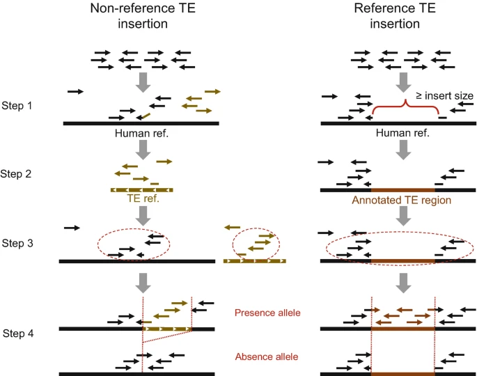
Figure 2. Overall strategies used for genotyping TE insertions using high-throughput sequence data. From Chen et al., 2022
- Many methods... The main limitation is that read length, and insert sizes are often smaller than the targeted TEs. Thus, long-read approaches or hybrid approaches (combining both) are more sensitive. Long reads and genome assemblies allows better detection of pME, but there is less data available, and starting from assembled genomes also depends on assembly quality (but this is improving very quickly!)
Table 1. Main methods available for pME calling

- One common limitation to most methods, is that the evaluation of the presence/absence of a TE, and their allelic state (homozygous or heterozygous) is based on mapping statistics over a reference genome, that only carries one of the two possible alleles (presence or absence of the TE). This is not only true for TEs, but it applies as well to all large (>50bp) structural variants (SV). In the recent years, pangenome-based approaches, and in particular graph-genomes allow to represent at the same time multiple alleles for a given loci. Several read mappers have been developed to be used with graph-genomes, which have dramatically increased the accuracy of SV and TE genotyping.

Figure 3. Pangenomes and Structural Variation.
GraffiTE is a pipeline that finds polymorphic mobile elements insertions (pME) by comparing genome assemblies or long read datasets to a reference genome, and then genotypes the discovered polymorphisms in read sets using a graph-genome representation of the pME. GraffiTE is made as a toolbox, containing different modules that can be combined to make the best of the user's data. GraffiTE is build as a Nextflow pipeline and relies on a Singularity image to handle the dependencies.
The pipeline is divided in 4 main steps:
- Step 1: Search of structural variants (SVs) between alternative assemblies (or long-reads sets) and the reference genome
- Step 2: Filtering of SVs to retain likely repeats (candidate pME)
- Step 3: Target site duplication (TSD) and TE-specific feature search
- Step 4: Graph-genotyping of pME using short or long read sets
In this tutorial, we will demonstrate the basic usage of GraffiTE by searching for pME between the individual HG002 and the reference genome GRCh38.p14 (hg38). We will first compare a diploid assembly of HG002 to the reference genome hg38 to identify candidate pME. The list of candidate pME will be used to create a TE graph-genome, where each pME sequence (TE-present haplotype) is represented a bubble (alternative path) in the graph. To validate each candidate pME, we will then map short reads (Illumina) onto the TE graph-genome, and infer their genotypes (i.e. heterozygosity) by comparing the read support between TE-absent (short paths) and TE-present (bubbles, long path) in the graph.
Most of these steps are automated in GraffiTE, and could be done using a single command. For clarity, we will break down the analysis in two major commands: 1) de-novo search for candidate pME and 2) graph-genotyping of each pME. Finally, we will discuss the outputs and how to interpret them.

Command 1: detection of candidate pME between the diploid assembly of HG002 and the reference genome (steps 1 through 3)

Command 2: Graph-genotyping of the pME (step 4)
At the end of this tutorial, you should be able to:
- Understand the general principle of the
GraffiTEmethod - Perform a simple analysis using assemblies to search for candidate pME and use short-reads to validate and genotype each polymorphism
- Explore and interpret the outputs of
GraffiTE
In order to speed-up the analyses during this tutorial, we will focus on the chromosome 22 only.
The following workflow represent the main steps and command of the pipeline

You can click here to reveal a more detailed workflow

Red paths indicate the workflow of the first command, while blue path indicate the workflow for the second command.
First, let's create a directory for this practical
mkdir practical3
cd practical3
The directory /home/ubuntu/Share/Practical_3/input contains all the files we will need for the execution of the program. We will first create a symlink to it, and check its content.
ln -s /home/ubuntu/Share/Practical_3/input/ input
tree input/input/
├── HG002.Illumina.fastq
├── HG002.assemblies.csv
├── HG002.mat.cur.20211005_chr22.fasta
├── HG002.pat.cur.20211005_chr22.fasta
├── HG002.reads.csv
├── hg38.p14.chr22.fa
└── human_DFAM3.6.fasta
-
Assemblies list:
HG002.assemblies.csv
This file indicate which assemblies to use, their path and name
cat input/HG002.assemblies.csvpath,sample
/home/ubuntu/Share/Practical_3/input/HG002.mat.cur.20211005_chr22.fasta,HG002.mat
/home/ubuntu/Share/Practical_3/input/HG002.pat.cur.20211005_chr22.fasta,HG002.pat
-
Reference genome:
hg38.p14.chr22.fasta -
Reads file list:
HG002.reads.csv
This file indicate which read set to use, their path and sample name In this case, there is only one read sample:
cat input/HG002.reads.csv
path,sample
/home/ubuntu/Share/Practical_3/input/HG002.Illumina.fastq,HG002
With short-reads, GraffiTE uses the program
Pangeniewhich maps read k-mers to the graph genome.Pangenierequires the input reads to be within a single file, thus in this example, R1 and R2 sets were concatenated. Due to time constraint, we will use a small read set, but will explore the results produced with a real read set with 10X coverage.
-
TE library:
human_DFAM3.6.fasta
This file contains the consensus sequences for human repeats (from DFAM)
These commands are needed to pull the GraffiTE repository (to do only once!)
apptainer remote add --no-login SylabsCloud cloud.sycloud.io
apptainer remote use SylabsCloud
If you get
FATAL: SylabsCloud is already a remoteit's all good, this means this was already set up.
nextflow run cgroza/GraffiTE --assemblies input/HG002.assemblies.csv --reference input/hg38.p14.chr22.fa --TE_library input/human_DFAM3.6.fasta --out results --mammal --genotype false --cpu 1 --stSort_t 1 --stSort_m "1G"
--stSort_t 1--stSort_m "1G": here we restrict the memory usage to spare the server, but there no need to use them in a normal setting. You may see a warning about the Singularity cache directory, but this is not an issue.
While the program is running, we can look at the command in details:
-
--assembliesindicate the path to the input tableHG002.assemblies.csv, which lists the path and sample name for each assembly of HG002. -
--reference: the path to the reference genome -
--TE_library: the path to the TE consensus sequences -
--out: the path where to write the outputs -
--mammal: will activate the search for LINE1 with 5' inversions, and SVA VNTR polymorphisms (see here) -
--genotype false: this will stop the pipeline before mapping the reads onto the TE graph-genome -
-with-singularity: indicate where the image hostingGraffiTEdependencies is located. It has a single-because it is aNextflowargument, while the others are pipeline-specific.
Nextflow subdivides each step of the pipeline into processes. While the pipeline runs, the status of each process is indicated.
You can click here to reveal the command 1 divided by `Nextflow` process (rather than steps)

Before going further we can take a brief look at the pipeline progress by following a variant through the annotation process (we will give a detailed description of the outputs in the [dedicated section](#outputs)):
-
Let's count the total number of SVs (including non-TE SVs) detected by
svim-asmafter analyzing both assembly (step 1):grep -v '#' results/1_SV_search/svim-asm_variants.vcf | sed 's/SVTYPE/\tSVTYPE/g;s/;SVMETHOD/\t/g' | cut -f 9 | sort | uniq -c
239 SVTYPE=DEL 402 SVTYPE=INS -
Now, lets count the number of variants retained after TE and TSD annotation (steps 2 and 3):
grep -v '#' results/3_TSD_search/pangenome.vcf | sed 's/SVTYPE/\tSVTYPE/g;s/;SVMETHOD/\t/g' | cut -f 9 | sort | uniq -c
38 SVTYPE=DEL 57 SVTYPE=INS -
let's look at one of these variants before annotating TEs (step 1)
grep -v '#' results/1_SV_search/svim-asm_variants.vcf | grep -w 'HG002.pat.svim_asm.DEL.1'
chr22 10536797 HG002.pat.svim_asm.DEL.1 GAAATATTTTTCCCTGGCCGGGCGCGGTGGCTCACGCCTGTAATCCCAGCACTTTGGGAGGCCGAGGCGGGTGGATCACGAGGTCAGGAGATCGAGACCATCCTGGCTAACAAGGTGAAACCCCGTCTCTACTAAAAATACAAAAAATTAGCCGGGCGCGGTGGCAGGCGCCTGTAGTCCCAGCTACTCGGGAGGCTGAGGCAGGAGAATGGCGTGAACCCGGGAAGCGGAGCTTGCAGTGAGCCGAGATTGCGCCACTGCAGTCCGCAGTCCGGCCTGGGCGACAGAGCGAGACTCCGTCTCAAAAAAAAAAAAAAAAAAAAAAAAAA G . PASS UPP=2;SUPP_VEC=11;SVLEN=-328;SVTYPE=DEL;SVMETHOD=SURVIVOR1.0.7;CHR2=chr22;END=10537125;CIPOS=0,0;CIEND=0,0;STRANDS=+- GT:PSV:LN:DR:ST:QV:TY:ID:RAL:AAL:CO 1/1:NA:328:0,0:+-:.:DEL:HG002.mat.svi_asm.DEL.1:GAAATATTTTTCCCTGGCCGGGCGCGGTGGCTCACGCCTGTAATCCCAGCACTTTGGGAGGCCGAGGCGGGTGGATCACGAGGTCAGGAGATCGAGACCATCCTGGCTAACAAGGTGAAACCCCGTCTCTACTAAAAATACAAAAAATTAGCCGGGCGCGGTGGCAGGCGCCTGTAGTCCCGCTACTCGGGAGGCTGAGGCAGGAGAATGGCGTGAACCCGGGAAGCGGAGCTTGCAGTGAGCCGAGATTGCGCCACTGCAGTCCGCAGTCCGGCCTGGGCGACAGAGCGAGACTCCGTCTCAAAAAAAAAAAAAAAAAAAAAAAAAA:G:chr22_10536797-chr22_10537125 1/1:NA:328:00:+-:.:DEL:HG002.pat.svim_asm.DEL.1:GAAATATTTTTCCCTGGCCGGGCGCGGTGGCTCACGCCTGTAATCCCAGCACTTTGGGAGGCCGAGGCGGGTGGATCACGAGGTCAGGAGATCGAGACCATCCTGGCTAACAAGGTGAAACCCCGTCTCTACTAAAAATACAAAAAATTAGCCGGGGCGGTGGCAGGCGCCTGTAGTCCCAGCTACTCGGGAGGCTGAGGCAGGAGATGGCGTGAACCCGGGAAGCGGAGCTTGCAGTGAGCCGAGATTGCGCCACTGCAGTCCGCAGTCCGGCCTGGGCGACAGAGCGAGACTCCGTCTCAAAAAAAAAAAAAAAAAAAAAAAAAA:G:chr22_10536797-chr22_10537125This file was made by comparing the variants found in each assembly. Columns 1 to 9 gives us information about each variant. Columns 10 and 11 are the genotype fields for each assembly. Because each assembly represents one haplotype, the genotype is always
1/1if the variant is found and./.otherwise. The program used to combine the variants from each assembly (SURVIVOR) also reproduce the reference and alternative alleles as originally detected for each assembly in the genotype field (This information will be removed in later outputs). The support vector (SUPP_VEC=in column 8) summarizes the variants presence/absence for each assembly with1(variant detected) or0(variant not detected) and will be carried over in the next steps. In this example, the variant is detected in both genomes, so the support vector is11. -
Now let's look at the same variant after the annotation steps:
grep -v '#' results/3_TSD_search/pangenome.vcf | grep -w 'HG002.pat.svim_asm.DEL.1'
chr22 10536797 HG002.pat.svim_asm.DEL.1 gaaatatttttccctggccgggcgcggtggctcacgcctgtaatcccagcactttgggaggccgaggcgggtggatcacgaggtcaggagatcgagaccatcctggctaacaaggtgaaaccccgtctctactaaaaatacaaaaaattagccgggcgcggtggcaggcgcctgtagtcccagctactcgggaggctgaggcaggagaatggcgtgaacccgggaagcggagcttgcagtgagccgagattgcgccactgcagtccgcagtccggcctgggcgacagagcgagactccgtctcaaaaaaaaaaaaaaaaaaaaaaaaaa g . PASS SUPP=2;SUPP_VEC=11;SVLEN=-328;SVTYPE=DEL;SVMETHOD=SURVIVOR1.0.7;CHR2=chr22;END=10537125;CIPOS=0,0;CIEND=0,0;STRANDS=+-;n_hits=1;fragmts=1;match_lengths=313;repeat_ids=AluYb8;matching_classes=SINE/Alu;RM_hit_strands=+;RM_hit_IDs=298;total_match_length=313;total_match_span=0.951368;mam_filter_1=None;mam_filter_2=None;TSD=AATATTTTTCCCT,aatatttttccct GT 1|0We can notice that several information have been added to the INFO field. We will detail them in a later section of this tutorial. Note that there is now only a single genotype column with the value
1|0. This is becauseGraffiTEwill use this file to generate the TE graph-genome. For each candidate pME, we will represent both the path with and without the TE, so both alleles must be present in the genotype field.
nextflow run cgroza/GraffiTE --graffite_vcf results/3_TSD_search/pangenome.vcf --reference input/hg38.p14.chr22.fa --reads input/HG002.reads.csv --out resultsHowever we will not actually run the command in order to keep the server alive!
You can click here to reveal the command 2 divided by Nextflow process

Since we didn't actually run the genotyping command, we have generated a "real" run using 10X of short reads. Let create a symlink to these results so it will look as if you had run the complete analysis.
ln -s /home/ubuntu/Share/Practical_3/results/4_Genotyping/ results/GraffiTE will output the results in the ./tutorial directory (--out tutorial). Each step of the pipeline produces at least one file in variant call format (VCF):
tree results/results/
├── 1_SV_search
│ ├── svim-asm_individual_VCFs
│ │ ├── HG002.mat.vcf # INS/DEL for the maternal genome vs reference
│ │ └── HG002.pat.vcf # INS/DEL for the paternal genome vs reference
│ ├── svim-asm_variants.vcf # merged VCF containing all INS or DEL
│ └── vcfs.txt # list of each individual VCF giving their order in the "Support Vector"
├── 2_Repeat_Filtering
│ ├── genotypes_repmasked_filtered.vcf # Filtered VCF containing INS or DEL with TE(s) >= 80% of the sequence
│ └── repeatmasker_dir # This directory contains the details of the RepeatMasker analysis
│ ├── ALL.onecode.elem_sorted.bak
│ ├── OneCode_LTR.dic
│ ├── indels.fa.cat
│ ├── indels.fa.masked
│ ├── indels.fa.onecode.out
│ ├── indels.fa.out
│ ├── indels.fa.out.length
│ ├── indels.fa.out.log.txt
│ ├── indels.fa.tbl
│ └── onecode.log
├── 3_TSD_search
│ ├── TSD_full_log.txt # Detailed test ouptout of the TSD search
│ ├── TSD_summary.txt # Summary (1 line per pME) output of the TSD search
│ └── pangenome.vcf # The fully annotated VCF with candidate pME and TSD(s).
└── 4_Genotyping
├── GraffiTE.merged.genotypes.vcf # Final annotated VCF with individual genotypes (1 genotype column per read set)
├── HG002_genotyping.vcf.gz # Individual VCF for each read set (here only one was used)
└── HG002_genotyping.vcf.gz.tbi # Index for each individual VCF
-
1_SV_search/svim-asm_variants.vcfcontains all the INS and DEL variants found between each assembly and the reference genome. It contains many SVs that are not TE-related. -
2_Repeat_Filtering/genotypes_repmasked_filtered.vcfcontains the INS and DEL variants for which at least 80% of their sequence is occupied by TEs. In spite of its name, it doesn't contain actual genotypes; rather, each variant's genotype is set to1|0in order to represent both alleles (TE-present/TE-absent) later in the graph. -
3_TSD_search: this file is the same as2_Repeat_Filtering/genotypes_repmasked_filtered.vcfwith an additional field for TSDs. -
4_Genotyping/GraffiTE.merged.genotypes.vcf: this is the final and most important output file. It contains all retained and annotated candidate pME with their genotypes based on the mapping of the read set.
Let's explore in more detail the file 4_Genotyping/GraffiTE.merged.genotypes.vcf. VCFs files start with a header with each line starting with a #.
- Column names:
grep 'CHROM' results/4_Genotyping/GraffiTE.merged.genotypes.vcf
#CHROM POS ID REF ALT QUAL FILTER INFO FORMAT <sample>
In our case, there is only one <sample> column. If more read sets are used (for example for multiple individuals), there will be one <sample> column per read set.
The details for each column, and each field within columns can be found in the main documentation.
To make sense of it, let's look at some entries in the output VCF. We will use the provided output file, generated with a complete set of reads (10X coverage)
-
Example 1: Alu deletion
grep -w 'HG002.pat.svim_asm.DEL.1' results/4_Genotyping/GraffiTE.merged.genotypes.vcf
chr22 10536797 HG002.pat.svim_asm.DEL.1 GAAATATTTTTCCCTGGCCGGGCGCGGTGGCTCACGCCTGTAATCCCAGCACTTTGGGAGGCCGAGGCGGGTGGATCACGAGGTCAGGAGATCGAGACCATCCTGGCTAACAAGGTGAAACCCCGTCTCTACTAAAAATACAAAAAATTAGCCGGGCGCGGTGGCAGGCGCCTGTAGTCCCAGCTACTCGGGAGGCTGAGGCAGGAGAATGGCGTGAACCCGGGAAGCGGAGCTTGCAGTGAGCCGAGATTGCGCCACTGCAGTCCGCAGTCCGGCCTGGGCGACAGAGCGAGACTCCGTCTCAAAAAAAAAAAAAAAAAAAAAAAAAA G . PASSUK=41;MA=0;AF=0.5;AK=41,0;CIEND=0,0;CIPOS=0,0;CHR2=chr22;END=10537125;SVLEN=-328;SVMETHOD=SURVIVOR1.0.7;SVTYPE=DEL;SUPP_VEC=11;SUPP=2;STRANDS=+-;n_hits=1;match_lengths=313;repeat_ids=AluYb8;matching_classes=SINE/Alu;fragmts=1;RM_hit_strands=+;RM_hit_IDs=298;total_match_length=313;total_match_span=0.951368;mam_filter_1=None;mam_filter_2=None;TSD=AATATTTTTCCCT,aatatttttccct GT:GQ:GL:KC 1/1:10000:-109.113,-100.6,0:20
This case represent a "classic" pME in the human population. Using the INFO column flags, we can see that this is an element from the AluYb8 family (repeat_ids=AluYb8), which belongs to the SINE/Alu order (matching_classes=SINE/Alu). The polymorphism length is 328 bp (SVLEN=-328), and represent a deletion relative to the reference genome (SVTYPE=DEL). The recognized TE sequence covers 95% of the variant sequence (total_match_span=0.951368).
The insertion strand is + (RM_hit_strands=+). GraffiTE later found a TSD for it: AATATTTTTCCCT (TSD=AATATTTTTCCCT,aatatttttccct). The TSD field represent both 5' and 3' TSD in case there are some mismatches.
STRANDS=+-should be ignored.
This polymorphism was initially discovered in both the maternal and paternal genomes during the first step of the pipeline according to the support vector (SUPP_VEC=11). The order in which the samples are represented in the support vector is given by their order in the file 1_SV_search.vcfs.txt.
Finally, upon read mapping, the polymorphism is confirmed for each haplotype (GENOTYPE column: 1/1). In the genotype field, 0 represent the reference allele, and 1 the alternative allele (fields REF and ALT respectively). Because the SVTYPE= is a DEL (Deletion), this means that HG002 is homozygous for the absence of this Alu element.
-
Example 2: LINE1 insertion with 5' Inversion
grep -w '5P_INV' results/4_Genotyping/GraffiTE.merged.genotypes.vcf
chr22 10643867 HG002.pat.svim_asm.INS.3 T TAAGAAAAATGTGGTTTTGATTTGCATTTCTCTGATGGCCAGTGATGATGAGCATTTCTTCATGTGTTTTTTGGCTGCATAAATGTCTTCTTTTGAGAAGTGTCTGTTCATGTCCTTCGCCCACTTTTTGATGGGGTTGTTTGTTTTTTTCTTGTAAATTTGTTTGAGTTCATTGTAGATTCTGGATATTAGCCCTTTGTCAGATGAGTAGGTTGCGAAAATTTTCTCCCATGTTGTAGGTTGCCTGTTCACTCTGATGGTAGTTTCTTTTGCTGTGCAGAAGCTCTTTAGTTTAATTAGAACTCATAGTTAAAACCACTATGAGATATCATCTCACACCAGTTAGAATGGCAATCATTAAAAAGTCAGGAAACAACAGGTGCTGGAGAGGATGCGGAGAAATAGGAACACTTTTACATTGTTGGTGGGACTGTAAACTAGTTCAACCATTGTGGAAGTCAGTGTGGCGATTCCTCAGGGATCTAGAACTAGAAATACCATTTGACCCAGCCATCCCATTACTGGGTATATACCCAAATGAGTATAAATCATGCTGCTATAAAGACACATGCACATGTATGTTTATTGCGGCACTATTCACAATAGCAAAGACTTGGAACCAACCCAAATGTCCAACAATGATAGACTGGATTAAGAAAATGTGGCACATATACACCATGGAATACTATGCAGACATAAAAAATGATGAGTTCATATCCTTTGTAGGGACATGGATGAAATTGGAAACCATCATTCTCAGTAAACTATCGCAAGAACAAAAAACCAAACACCGCATATTCTCACTCATAGGTGGGAATTGAACAATGAGATCACATGGACACAGGAAGGGGAATATCACACTCTGGGGACTGTGGTGGGGTTGGGGGAGGGGGGAGGGATAGCATTGGGAGATATACCTAATGCTAGATGACACATTAGTGGGTGCAGCGCACCAGCATGGCACATGTATACATATGTAACTAACCTGCACAATGTGCACATGTACCCTAAAACTTAGAGTATAATAAAAAAAAAAAAA . PASS UK=92;MA=0;AF=0.5;AK=10,82;CIEND=-7,0;CIPOS=0,0;CHR2=chr22;END=10643867;SVLEN=1038;SVMETHOD=SURVIVOR1.0.7;SVTYPE=INS;SUPP_VEC=11;SUPP=2;STRANDS=+-;n_hits=2;match_lengths=296,731;repeat_ids=L1HS,L1HS;matching_classes=LINE/L1,LINE/L1;fragmts=1,1;RM_hit_strands=C,+;RM_hit_IDs=659,659;total_match_length=1027;total_match_span=0.98845;mam_filter_1=5P_INV:plus;mam_filter_2=None;TSD=AGAAAAAT,agaaaaat GT:GQ:GL:KC 0/1:10000:-126.12,0,-72.03:16
This example is similar to the previous one, but with two major differences:
- The pME is an insertion relative to the reference genome
- This pME is a special case where the LINE1 element inserts with a 5' inversion: this given by the flag
mam_filter_1=5P_INV:plus. This is quite common for LINE1, and may represent up to 25% of LINE1 insertions in humans.
You can notice that in this particular case, GraffiTE reports
n_hits=2. Indeed, when this type of insertion occurs,RepeatMasker-- the program used to identify TEs -- produces two consecutive hits for the same sequence (repeat_ids=L1HS,L1HS;matching_classes=LINE/L1,LINE/L1) however, we can see that the first hit appears to be on the complementary strand (C) while the second on the positive strand (+). In reality, the TE is inserted in the+strand, as we can see the poly-A tail in 3'. Because we used the argument--mammal,GraffiTEautomatically search for this specific pattern and indicatemam_filter_1=5P_INV:plus.
-
Example 3: false positive (not a pME)
grep -w 'HG002.pat.svim_asm.INS.283' results/4_Genotyping/GraffiTE.merged.genotypes.vcfchr22 50800276 HG002.pat.svim_asm.INS.283 G GATTTCAGCCATGAATCAGGCATAAATATTCTGACGGTTAATTTTAGACATCAACTTGACTGGATTAAGGGACACACATAGCTGGTCAAACACGATTTCAGCCATGAATCAGGCATAAATATTCTGATGGTTAATTGTAGACATCTACTTGACTGGATTGAGAGACACACATAGCTGGTCAAACACGATTTCAGCCATGAATCAGGCATAAATATTCTGATGGTTAATCGTAGACGTCTACTTGACTGGATTGAGAGACACACATAGCTGGTCAAACACGATTTCAGCCATGAATCAGGCATAAATATTCTGATGGTTAATTTTAGACATCTACTTGAGTGGATTGAGAGACACACATAGCTGGTCAAACACAATTTCAGCCATGAATCAGGCATAAATATTCTGATGGTTAATTTTAGACATCTACTTGAGTGGATTGAGAGACACACATAGCTGGTCAAACAATTTCAGCCATGAATCAGGCATAAATATTCTGACGGTTAATTTTAGACATCTACTTGAGTGGATTGAGAGACACACATAGCTGGTCAAACACA . PASS UK=0;MA=0;AF=0.5;AK=0,0;CIEND=0,0;CIPOS=0,0;CHR2=chr22;END=50800276;SVLEN=556;SVMETHOD=SURVIVOR1.0.7;SVTYPE=INS;SUPP_VEC=01;SUPP=1;STRANDS=+-;n_hits=6;match_lengths=92,92,92,92,90,60;repeat_ids=MLT2B5,MLT2B5,MLT2B5,MLT2B5,MLT2B5,MLT2B5;matching_classes=LTR/ERVL,LTR/ERVL,LTR/ERVL,LTR/ERVL,LTR/ERVL,LTR/ERVL ;fragmts=1,1,1,1,1,1;RM_hit_strands=+,+,+,+,+,+;RM_hit_IDs=656,656,656,656,656,657;total_match_length=518;total_match_span=0.929982;mam_filter_1=None;mam_fil ter_2=None GT:GQ:GL:KC 1/1:54:-11.5131,-5.456,-1.521e-06:7In this case, we can identify some clues indicating that this polymorphism is probably not due to a transposition, but has been retain due to spurious hits on the TE library we used:
- There are a total of 6 hits, and each hit is very small (< 100 bp). All hits are from the same consensus sequence (
MLT2B5) and in the same orientation. This suggest a tandem repeat expansion (we could investigate further looking at for the sequenceHG002.pat.svim_asm.INS.283in the RepeatMasker outputsresults/2_Repeat_Filtering/repeatmasker_dir/indels.fa.onecode.out). - The consensus sequence of
MLT2B5correspond to the LTR region of an element of the class LTR/ERVL, which size is 717 bp. - ERVL belongs to an older group of endogenous retroviruses which have been a long time inactive in the human lineage. There is no experimental evidence of ERVL polymorphism in the human population.
- There are a total of 6 hits, and each hit is very small (< 100 bp). All hits are from the same consensus sequence (
As we have seen in the previous examples, it is important to form hypotheses about what type of pME we expect in order to reduce the number of false positives. In humans, only 3 superfamilies of TEs are known to be active: Alu, LINE-1 and SVA. Additionally, one family of endogenous retrovirus, HERV-K is known to display a small amount of polymorphisms between individuals. Other ERVs are fixed in the human lineage.
Furthermore, we need to take into account a special case for SVA elements. These elements contain a region with a variable number of tandem repeats (VNTR). Upon insertion, the VNTR region can later undergo changes in copy number, in a way comparable to microsatellites. Thus, even when a given individual is homozygous for the presence of an SVA insertion, one allele may be longer than the other due to variability in the VNTR region (see here for a clinical example). Using the --mammal argument, we asked GraffiTE to distinguish between insertion polymorphism (TE either present or absent) and VNTR polymorphism. These cases are reported with the flag mam_filter_2=VNTR_ONLY.
Accordingly, we will take these hypothesis into account while parsing the results.
-
Counting pME
We will now count the number of likely pME in our dataset. The criteria are:
- The TE is either Alu (SINE/Alu), LINE-1 (LINE/L1), SVA (Retroposon/SVA) or HERVK (LTR/ERVK). (
grep#1) - The number of hits should be 1, except in the case of LINE-1 5' inversions (
grep#2) - SVA with
VNTR_ONLYare not counted as pME (grep#3)
grep -v '#' results/4_Genotyping/GraffiTE.merged.genotypes.vcf | \
 grep 'Alu\|L1\|SVA\|ERVK' | grep 'n_hits=1;\|5P_INV' | grep -v 'VNTR_ONLY' | \
 sed 's/repeat_ids=/\t/g;s/;matching_classes=/\t/g;s/;fra/\t/g' | \
 cut -f 9-10 | sort | uniq -c
- The TE is either Alu (SINE/Alu), LINE-1 (LINE/L1), SVA (Retroposon/SVA) or HERVK (LTR/ERVK). (
1 AluSc8 SINE/Alu 1 AluSg4 SINE/Alu 1 AluSp SINE/Alu 1 AluSx3 SINE/Alu 1 AluSx4 SINE/Alu 2 AluSz SINE/Alu 1 AluSz6 SINE/Alu 1 AluY SINE/Alu 11 AluYa5 SINE/Alu 10 AluYb8 SINE/Alu 1 AluYh3 SINE/Alu 1 AluYi6 SINE/Alu 1 AluYk11 SINE/Alu 1 AluYk2 SINE/Alu 1 AluYk4 SINE/Alu 4 L1HS LINE/L1 1 L1HS,L1HS LINE/L1,LINE/L1 <-- notice here, 2 hits, one for the reverse (inversion), and 1 for the forward bit. 1 L1M4 LINE/L1 1 L1PA13 LINE/L1 1 L1PA3 LINE/L1 1 SVA_D Retroposon/SVA 2 SVA_F Retroposon/SVA
or summarized per superfamily:

```sh
grep -v '#' results/4_Genotyping/GraffiTE.merged.genotypes.vcf | \
 grep 'Alu\|L1\|SVA\|ERVK' | grep 'n_hits=1;\|5P_INV' | grep -v 'VNTR_ONLY' | \
 sed 's/repeat_ids=/\t/g;s/;matching_classes=/\t/g;s/;fra/\t/g' | \
 cut -f 10 | sort | uniq -c
      7 LINE/L1
      1 LINE/L1,LINE/L1
      3 Retroposon/SVA
     35 SINE/Alu
-
Note that
LINE/L1,LINE/L1correspond to the L1 with a 5' inversion (two hits). -
We observe the ratio Alu/L1/SVA to be 35/8/3 which is consistent with the literature, e.g.: Sudmant et al., 2015 and Watkins and et al., 2020.
Figure 1. From Watkins et al., 2020.
-
We also fund a little more LINE1 and SVA than reported in the reference above: this is likely because this survey was conducted only with short-reads, which are prone to miss longer elements such as LINE1 and SVA (1000-5000 bp). Using high-quality genome assemblies established from long-read sequences, we were able to increase the sensitivity of pME detection for these elements.
-
Count pME with TSD
Target site duplications (TSDs) are a hallmark of transposition for many TE families. TSDs can vary depending on the TE family. For human retrotransposons such as Alu, L1 and SVA, the target site duplication can be variable in size. We can look for pME identified with a TSD with the following command:
grep -v '#' results/4_Genotyping/GraffiTE.merged.genotypes.vcf | \
   grep 'Alu\|L1\|SVA\|ERVK' | grep 'n_hits=1;\|5P_INV' | grep -v 'VNTR_ONLY' | \
   grep 'TSD=' | \
   sed 's/repeat_ids=/\t/g;s/;matching_classes=/\t/g;s/;fra/\t/g;s/TSD=/\tTSD=/g' | \
   cut -f 1,2,9-10,12
chr22 10536797 AluYb8   SINE/Alu TSD=AATATTTTTCCCT,aatatttttccct
chr22 10643867 L1HS,L1HS   LINE/L1,LINE/L1   TSD=AGAAAAAT,agaaaaat
chr22 10673603 AluYi6   SINE/Alu TSD=TGCTTTCCCAAT,TGCTTTCCCAAT
chr22 16164937 AluYa5   SINE/Alu TSD=TGAGTGAGTTTCTT,tgagtgagtttctt
chr22 17224400 AluYb8   SINE/Alu TSD=ACAAGTGCTAATAA,acaagtgctaataa
chr22 17616750 AluYa5   SINE/Alu TSD=AAGAGTCATACAAGA,aaGAGTCATACAAGA
chr22 17653856 SVA_F Retroposon/SVA TSD=AAAAATTGTTTAT,AAAAATTGTTTAT
chr22 17801130 AluYa5   SINE/Alu TSD=CCTGAGTTTCC,CCTGAGTTTCC
chr22 19223372 L1HS  LINE/L1  TSD=AAAAACCACCTATGCTG,Aaaaaccacctatgctg
chr22 21236136 AluSz SINE/Alu TSD=atgg,ATGG
chr22 23530481 AluYb8   SINE/Alu TSD=GAAAGCTGGGGAA,GAAAGCTGGGGAA
chr22 28781333 AluYa5   SINE/Alu TSD=gtttTGTTT,Gttttgttt
chr22 33673818 AluSz6   SINE/Alu TSD=CTGGGTTA,ctgggTTA
chr22 34034609 AluYb8   SINE/Alu TSD=AAATGGAAC,aaatggaac
chr22 35631629 AluYa5   SINE/Alu TSD=GAAAACACA,GAAAACACA
chr22 35673756 AluYa5   SINE/Alu TSD=AAAAAGGGGAGGC,Aaaaaggggaggc
chr22 39211647 AluYb8   SINE/Alu TSD=AAAAAGTCTGTGGC,aaaaaGTCtgtggc
chr22 41744474 AluYa5   SINE/Alu TSD=TATGATTTTT,TATGATTTTT
chr22 42818816 AluYa5   SINE/Alu TSD=ttTCT,tttct
chr22 43153319 AluYb8   SINE/Alu TSD=GCTTATTTGTGT,gcttatttgtgt
chr22 45479135 AluYb8   SINE/Alu TSD=TATTATAAA,TATTATAAA
chr22 48249398 AluYa5   SINE/Alu TSD=AGATTGCGCCTT,agaTTGCGCCTT
To know more about how
GraffiTEsearches for TSD, you can consult the documentation here.

Nextflow creates a work/ directory which includes all the intermediate files. This is useful to resume an interrupted job. When successful, it is recommended to remove this directory to save on storage.
rm -rf work/
🎉 Congratulations! You now know how to use GraffiTE!